Lessons on the use of R statistical software program [THIS PAGE IS UNDER DEVELOPMENT]

R graphics and visualization tools for exploring the Fisher’s Iris flower data set

One of the most unique and powerful aspects of R programming language is its ability to create a large variety of statistical graphs. We can draw bar graphs, line charts, pie charts, histograms, scatter plots, density plots, box-and-whisker plots, time-series graphs, lattice graphs, heat maps, and probability plots. These graphs are excellent means for demonstrating and visualizing data. One of the best ways to understand the power of R’s graphical tools is to see them in action. This lesson is the first of a series of lessons to demonstrate the use of R for graphics and data visualization. In each of the following two examples, please mouse over the image to see a larger version of the plot and click on the source code link to get to the R code utilized to generate the graph.

Graphical representation of four numerical variables in a single frame

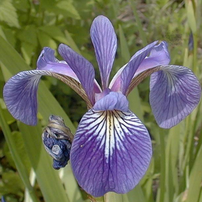
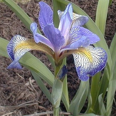
The Iris flower data set, also called the Fisher’s Iris data set, is a data set in four variables introduced by Sir Ronald Fisher in 1936 as an example of discriminant analysis. It is available in the R datasets package. As described in the R documentation, the Iris data set gives the measurements in centimeters of the variables sepal length and width and petal length and width, respectively, for 50 flowers from each of three species of iris flowers. The species are iris setosa, versicolor, and virginica. Images of these species are presented below.

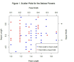
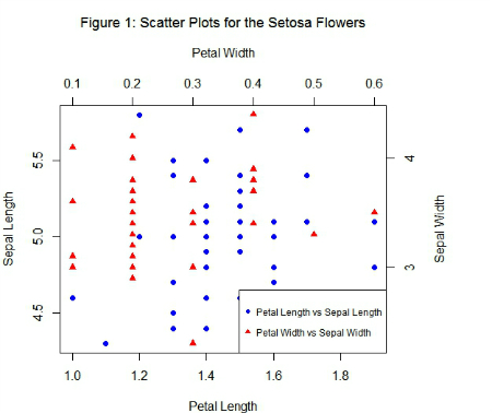Four-variable scatter plot in a single frameBased on the combination of the variables petal length, petal width, sepal length, and sepal width, Fisher developed a linear discriminant model to distinguish the species of iris flowers from each other. To describe the data set and examine the relationship between the four variables, we may obtain, for instance, a graphical representation of the data for the setosa flowers on these four variables in a single frame. We can construct a scatter plot of petal length and sepal length, and, then, superimpose this graph with the scatter plot of petal width and sepal width. These two scatter plots, presented in a single graph, can easily be obtained by using the R plot() function. If you are interested in the R code and all the steps to get this graph, please click here. The resulting graph is displayed in Figure 1. In a similar manner, we can construct scatter plots for the four variables in a single frame for the versicolor and virginica species.

Scatter plot matrix for the Iris data set

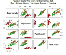
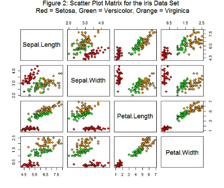Scatter plot matrix for the Iris data set There are several R functions that can be used to create a matrix of scatter plots for multivariate data. Among them, we can cite the pairs(), scatterplotMatrix(), and plotmatrix() functions of the graphics, car, and ggplot2 packages, respectively. For this example, we will use the pairs() function for exploring relationships among the variables in the data set Iris. The R pairs() function allows us to easily obtain scatter plots of the data by the three species of iris flower (setosa, versicolor, and virginica). Figure 2 shows the scatter plot matrix for the data, obtained with the pairs() function. To see the R code utilized to generate the graph, click here. To bring up a pop up window showing an amplified version of the graph, mouse over the figure.